manual

Foreword

mucha implements a simple workflow for multiscale comparison and heterogeneity analyses.

Put briefly, the idea is to obtain a summary statistic for all pixels of a single (MHM) or two (CMP) landscapes, using a moving window approach, and for with a varying window size. Then composite map and profile plot are calculated, so that multiscale patterns can be detected, analysed and displayed.

The primary goal of the CMP R package is to port the MHM and CMP softwares by Gaucherel and colleagues to R.

These softwares were written in Java and are no longer maintained.

This R port is a thin wrapper on top of the excellent terra package and notably terra::focal and terra::focalPairs functions.

The full references of the two articles by Gaucherel and colleagues follow:

Gaucherel, C. (2007) Multiscale heterogeneity map and associated scaling profile for landscape analysis, Landscape and Urban Planning 82(3) 95-102. doi: 10.1016/j.landurbplan.2007.01.022
Gaucherel, C., Alleaume, S. and Hély, C. (2008) The Comparison Map Profile method: a strategy for multiscale comparison of quantitative and qualitative images. IEEE Transactions on Geoscience and Remote Sensing 46 (9): 2708-2719 doi: 10.1109/TGRS.2008.919379

Package name is also a tribute to the work of Alfons Mucha.

Install and load `mucha`

Get it

You can install the last released version on CRAN straight for R console with with:

install.packages("mucha")

If you prefer to work with the very last (development) version you can install it with GitHub with:

pak::pak("vbonhomme/mucha")

Load it

Then, you can load mucha and terra packages. terra is optional but you are very likely to need it anyway.

library(mucha)   
library(terra)
#> terra 1.8.86

Online manual

The package documentation, produced by pkgdown in available on package’s homepage: https://vbonhomme.github.io/mucha
Issues, bug reports, feature request, etc. can be made at https://github.com/vbonhomme/mucha.

MHM and CMP speed dating

plop

Import and prepare data

From images

import_raster can be used to import any image format into mucha. More largely, any SpatRaster(), for example obtained with rast function in terra.

We recommend using .tif for source images and not compressed formats like .jpg that are very likely to produce artifacts even at the highest quality.

From text formats

If your raster is saved as a .txt (or equivalent such as .csv ,etc.) you can also use import_txt() which is a thin wrapper on top of read.table.

More generally, MHM() and CMP() functions will accept any raster as SpatRaster (see above). If this is not the case, try to use rast() on it.

Example data

Some example landscapes are bundled with the package and can be imported with import_example().

The full list of examples is available when passing the latter with no argument (import_example(). Once you made your choice, you can import it with its name.

We will continue with these examples for portability purposes but everything shown here should be available with your own images.

import_example() # all example files
#> Available example files to call with import_example('one_of_those_below'):
#> l1.tif
#> l1.txt
#> l2.tif
#> l2.txt
l1 <- import_example("l1.tif")
l1 %>% raster_summary()
#> >>> [801x600] raster (likely categorical)
#> >>> with following (9) classes: 1, 4, 9, 11, 12, 13, 14, 15, 16
#> >>> 349850 NA (72.8%) among 480600 values

Raster preparation

`p()` to plot your landscape(s)

All raster operations allowed by terra can be done on your own raster since mucha uses nothing much than SpatRaster class.

For example, you can use a plot() to visualize your raster but the built-in p() function is better suited for our needs:

l1 %>% p()

l1 %>% p(palette="Geyser")

l1 %>% p(palette="RdYlGn")

For palette enthusiasts, the full list is available there: hcl.pals(). Any vector of colors is also accepted.

qualitative versus continuous raster

Depending on the nature of your layers, they may be by nature categorical/qualitative (for example land occupations) or continuous/quantitative (digital elevation map, rainfall records, etc.)

Should you want to explicitly declare qualitative layers as factors, you can use raster_reclare_classes to turn your values into factor, with an optionnal data.frame as follows:

# enforce qualitative
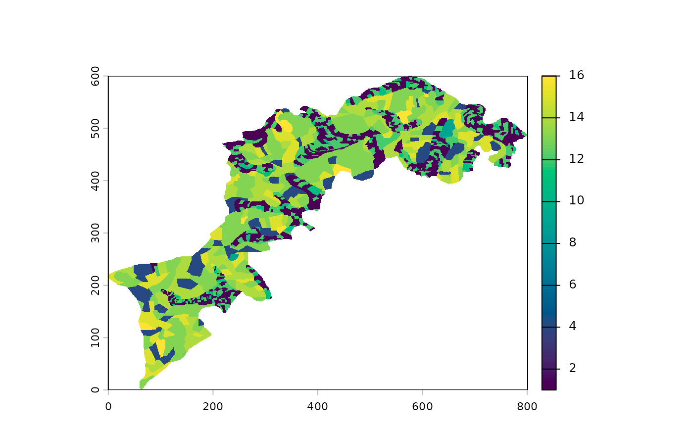
l1 %>% raster_declare_classes() %>% p()

# for an explicit declaration with class names
# we will build a data.frame
# first extract all values
values <- l1 %>% values %>% na.omit() %>% as.numeric() %>% unique() %>% sort()
# and their correspondance (dummy)
labels <- c("shrub", "corn", "habitations", "forest1", "forest2", "forest3", "cereal1", "cereal2", "cereal3")
# build the data.frame
df <- data.frame(value=values, label=labels)
# and now
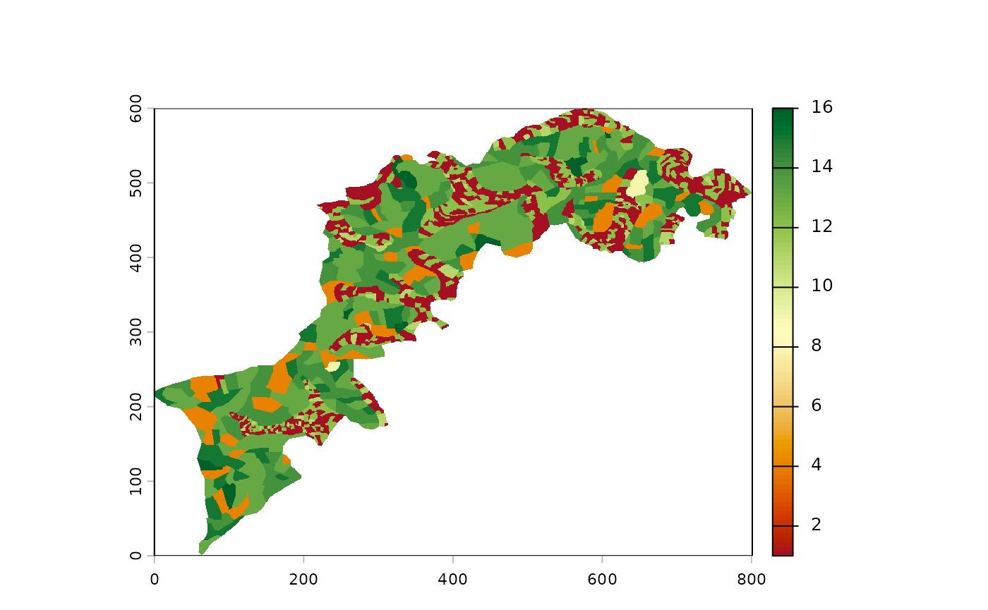
l1 <- l1 %>% raster_declare_classes(df)
p(l1)

A nice side-effect is to have a better plot now. That you can push further with a dedicated color scheme that can be passed to p:


# a nice land occupation color scheme
land_occupations <- c("yellow", "gold", "orange",
                      "palegreen", "palegreen2", "palegreen3",
                      "slateblue", "slateblue4", "slategray")
#' and now a nice plot we have
x %>% p(palette=land_occupations)

For those not familiar with the forward pipe %>% (or |>), that may get confused with the use of one or the other syntax, let’s just say that p(x) is equivalent to x %>% p(). When more than a single function is called, it helps defining more readable pipes. Read ?pipeOp` for more informations.

Minify your landscape to speed up calculations

One very useful function is raster_resample(). Given MHM() and CMP() imply huuuuge calculations, a nice approach can be to setup and try/error your analyses with a minified version of your landscape(s), then run the final one on the pristine full res version.

That’s exactly what we will do here, to speed up calculations. Note that below we exemplify how to use different color palette in p().

# see hcl.pals() for a full list of palettes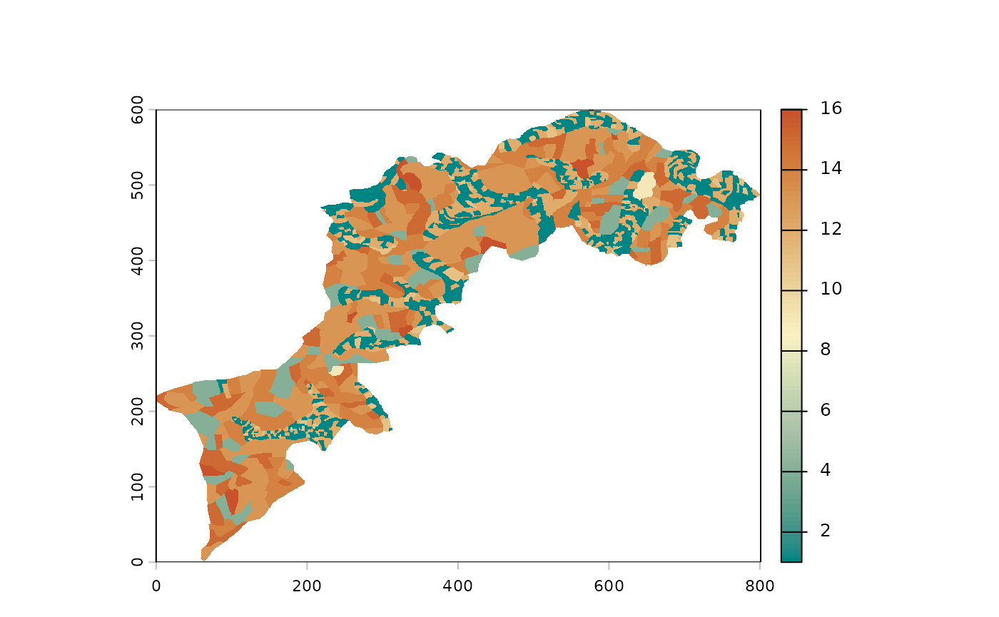
l1 %>% raster_resample(0.1) %>% p(palette="Earth")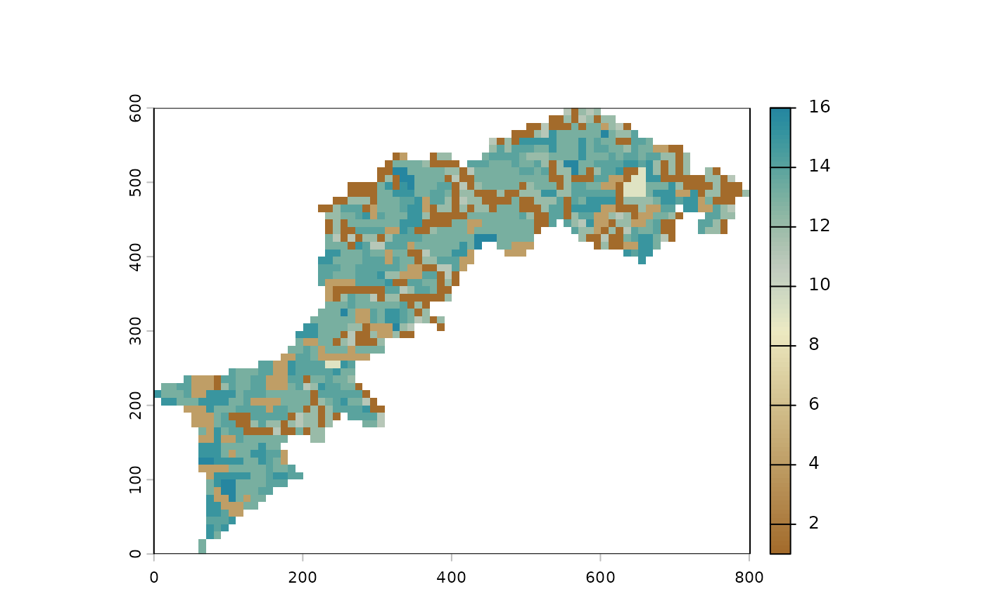

Other raster helpers

More generally, all raster_* functions implement common basic manipulations on rasters. See ?raster_helpers.

For example, to explicitly declare your NAs, use raster_declareNA().

Some other examples:

raster_likely_categorical(l1) # a non perfect heuristic based on the number of classes. See ?cats
#> [1] TRUE
raster_classes(l1) # class names. again to declare name explicitly, see ?cats
#> [1] "1"  "4"  "9"  "11" "12" "13" "14" "15" "16"

As stated before, you can use terra functions and/or combine with mucha’s ones:

x <- values(l1) # extract all pixel values
signif(100*table(na.omit(x)) / length(na.omit(x)), 3) # class percentages for non NA pixels
#> 
#>      1      4      9     11     12     13     14     15     16 
#> 17.800 10.200  0.699  2.780 11.100 26.900 18.000 10.600  1.920

MHM: multiscale statistics on a single landscape

Base usage

Vanilla MHM() runs with candid default values (see ?MHM):

focal function is mean
window is c(3, 13, 23)
with a circular kernel

l1_mhm <- l1 %>% MHM()

fun can be passed with any function returning a scalar, ie a numeric of length 1, ie a single value. See ?mhm_funs for richness, simpson and shannon indices, etc. and also contagion and kappa_index for categorical landscapes.

window must only contain odd numbers. odd_floor is your friend to do so. window_broad and window_linearpixels are helpers to obtain (often) interesting window size range.

*kernel can be passed with one of kernel function (ie to have square, gaussian, etc.). With kernel_gaussian, only sum is allowed by terra.

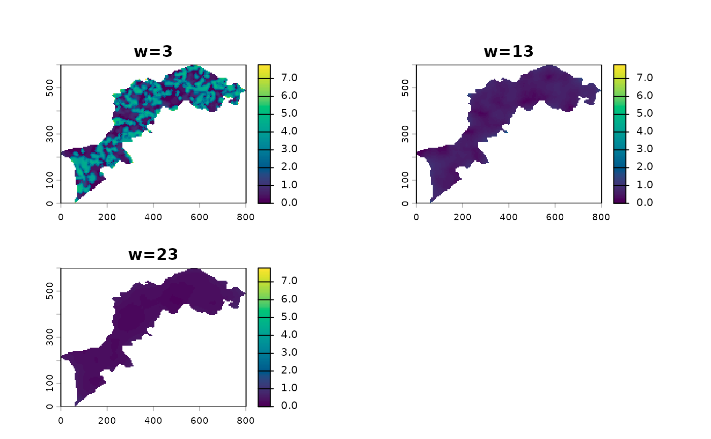
Let’s change a bit default values to i) change the window range and ii) use richness (ie count the number of classes). Before that, we resample so that calculations are not too long while we’re still tuning our analyses.

l1_lite <- raster_resample(l1, width = 120)
w <- window_linearpixels(l1_lite, steps = 6)
l1_mhm <- MHM(l1_lite, 
              fun=richness,  
              window = w)

Monoscale maps, multiscale map and profile plot

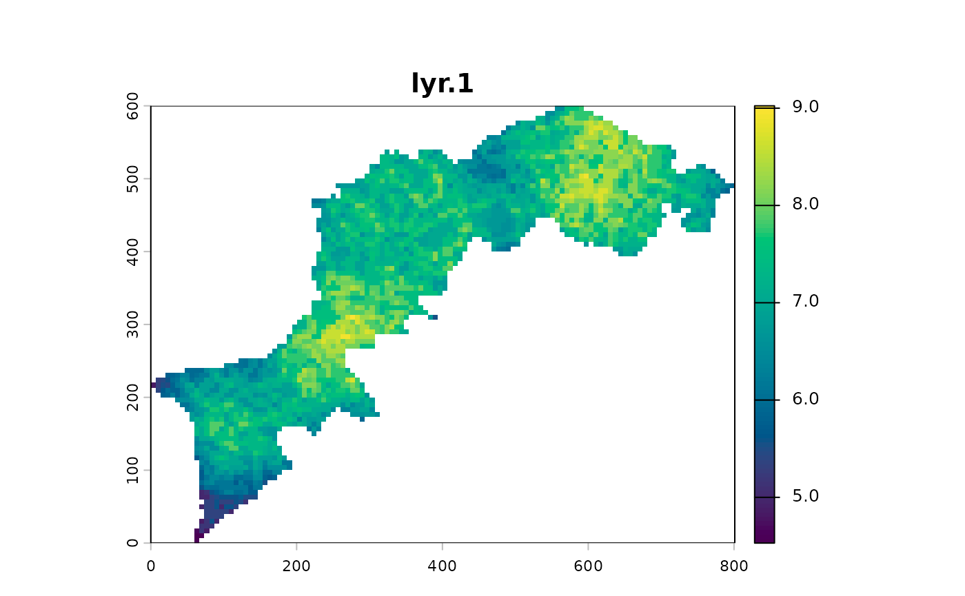
The object you obtain is also a SpatRaster on which you can access particular layers with say l1_mhm[[2]]. But it is probably more interesting to have a look to all monoscale maps at once:

l1_mhm %>% p()

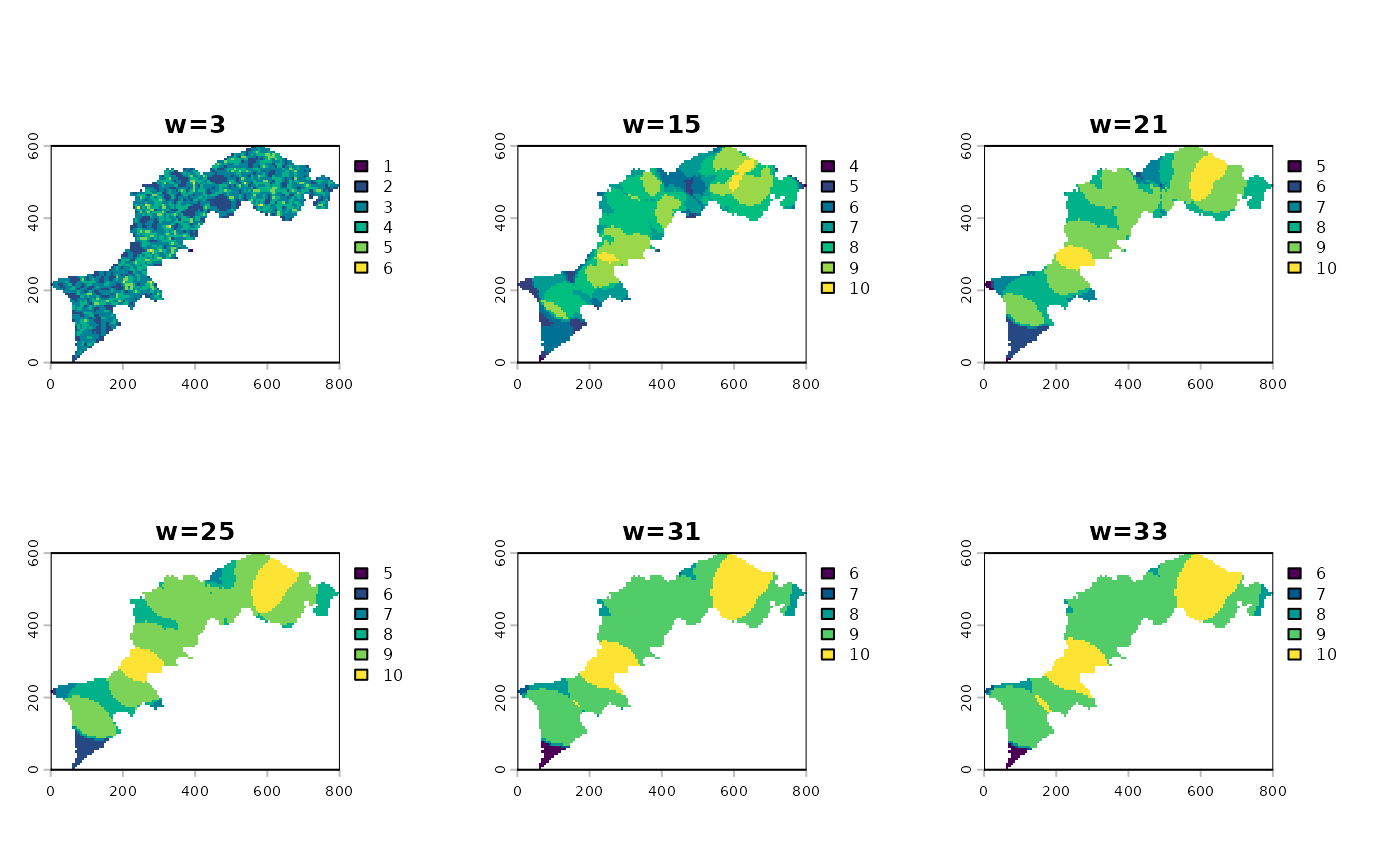
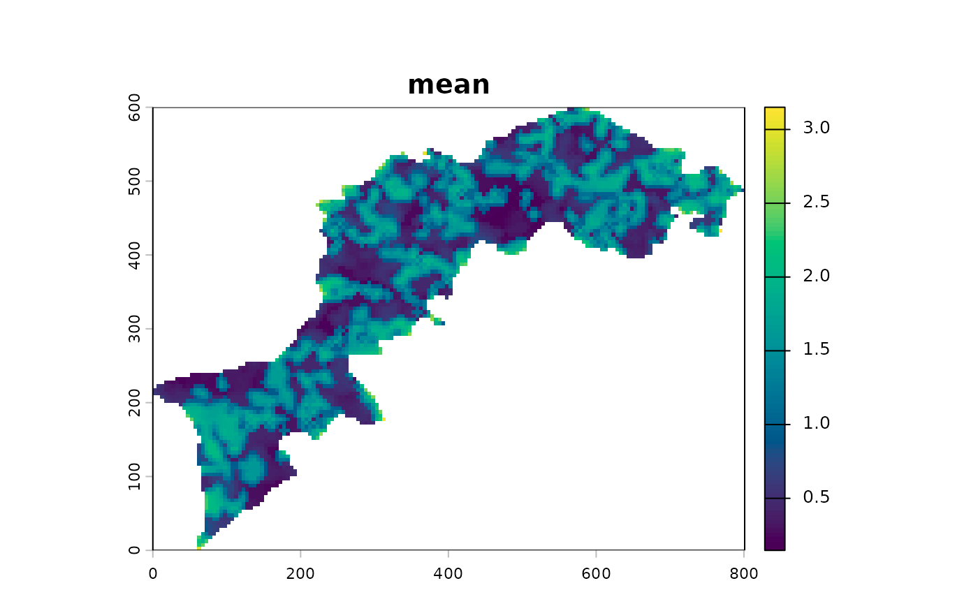
You can all apply one more function accross all layers and calculate a composite map, aka a multiscale map:

l1_mhm %>% app(mean) %>% p()

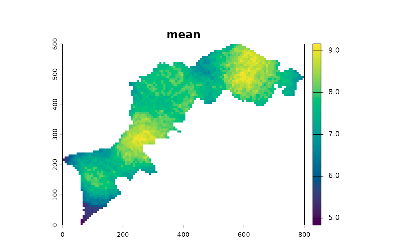
At this step, a geometric mean exacerbates the gradients:

l1_mhm %>% app(gmean) %>% p()

You can calculate the profile plot and calculate a global summary using two functions per window size and plot it.

l1_mhm %>% ms_profile() # mean ± SD by default

l1_mhm %>% ms_profile(summary_fun=median, error_fun = sd, ylab="median ± sd") # mean ± SD by default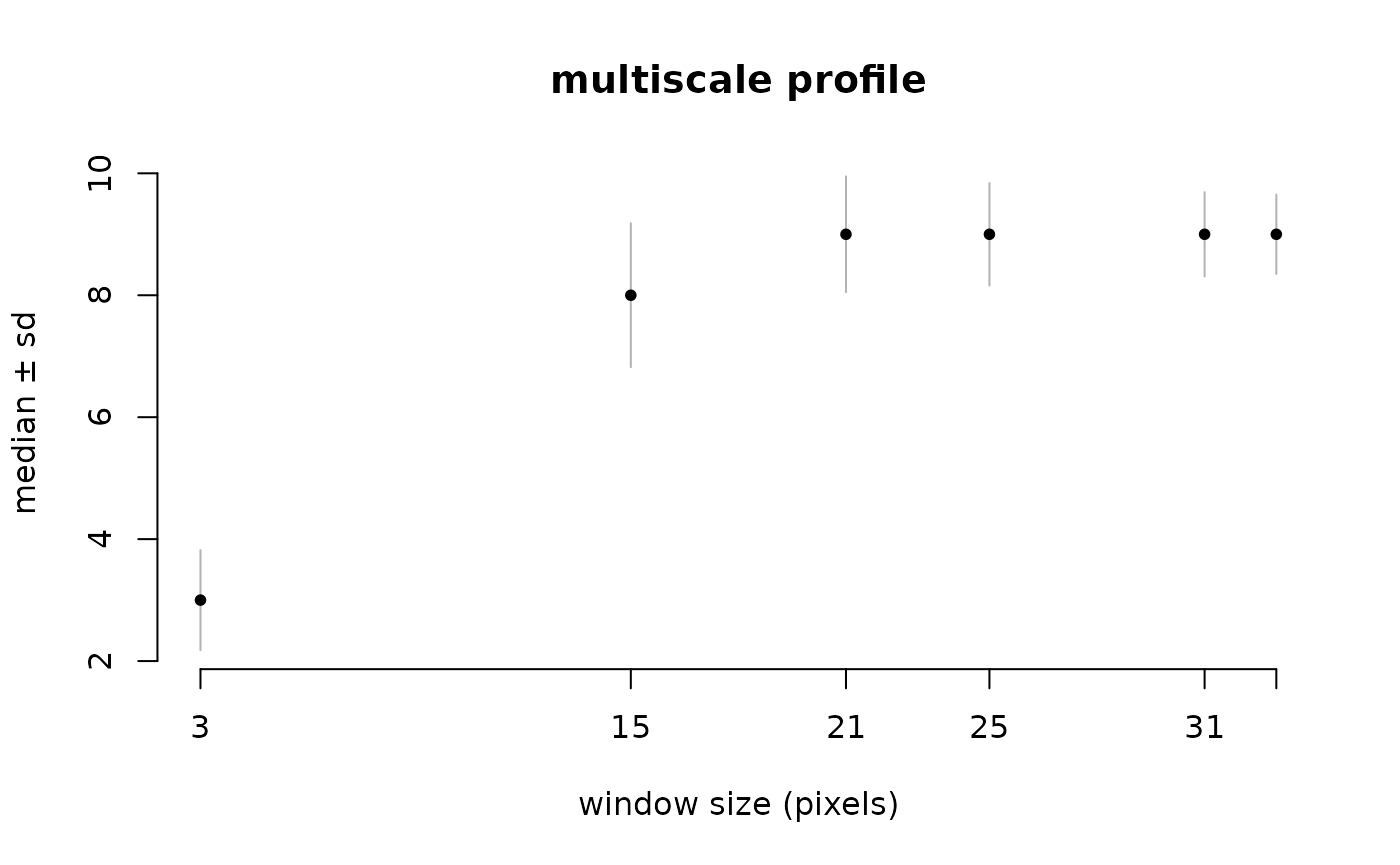

CMP: multiscale statistics on a pair of rasters

CMP works almost exactly the same except that it uses two landscapes and consequently uses appropriate (and other) functions (See ?cmp_funs).

That being said, what follows should sound familiar.

# let's iport the two example rasters from CMP paper
l1 <- import_example("l1.tif") %>% raster_resample(0.2)
l2 <- import_example("l2.tif") %>% raster_resample(0.2)

# let's plot them
c(l1, l2) %>% p()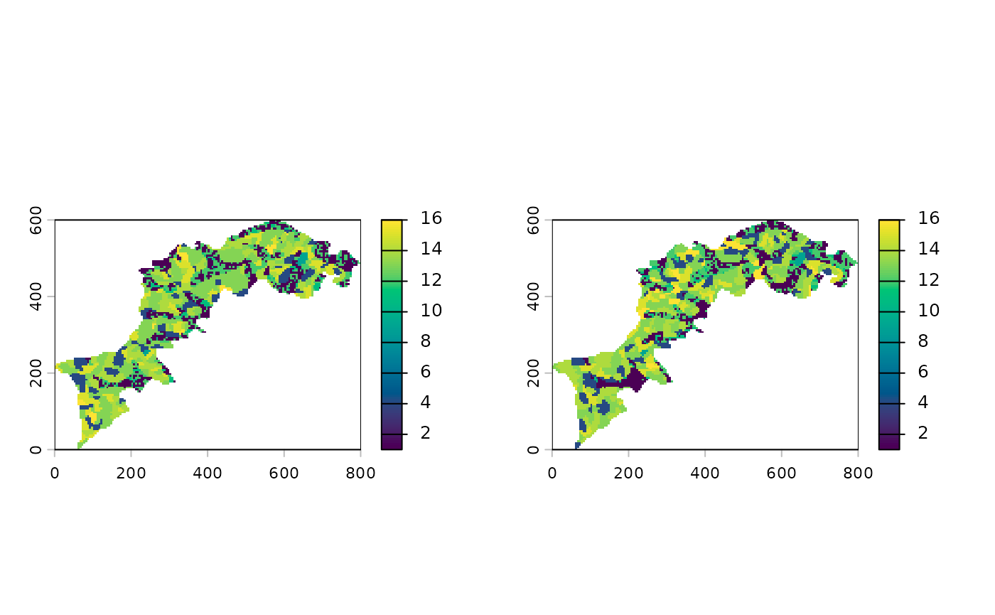

Now we will calculate CMP using a bare correlation.

l12_cmp <- CMP(l1, l2, fun=dist_euclidean)

And again, show the different summaries starting with the monoscale maps, then the profile plot and finally the multiscale map:

l12_cmp %>% p()

l12_cmp %>% ms_profile()

l12_cmp %>% app(mean, na.rm=TRUE) %>% p()

Export results

Have a look to export_image and export_txt functions.

Otherwise follow terra guidelines for manipulation the stack of monoscales layers.

Going further

Can I use custom functions for MHM and CMP?

Yes, have a look to function definitions, eg shannon or cor_pearson (no parentheses to access function definition) and mimic it. For both MHM and CMP, do not forget ... as an argument. For CMP, think of declaring x and y as arguments.

Can I write my own `ms_profile` function, eg in ggplot2?

Sure, and ms_profile_df may help to do so.

Should you have any idea, suggestions, etc. feel free to contact me: bonhomme.vincent@gmail.com