Monoscale plot after an MHM/CMP

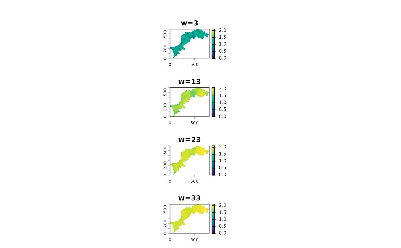
For what we have to represent, this is a better plot for SpatRaster than base terra's plot. The main benefit being sharing the legend across monoscale maps.

Usage

p(
  x,
  palette = "Viridis",
  asp = 1,
  ncol = NULL,
  title,
  multi_title,
  global_range = TRUE,
  ...
)

Arguments

x

a SpatRaster typically obtained after MHM/CMP

palette

one of grDevices::hcl.colors palette description (default to viridis)

asp

target aspect for the layout (default to 1 that is a square)

ncol

integer number of columns for the layout, if provided asp is ignored

title

for each plot, if missing use names(x)

multi_title

for the general plot (eg when more than one layer)

global_range

logical, default to TRUE, whether to use a global range for all layers

...

additional parameters to single plot call

Examples

# first calculate a small and simple MHM
l <- import_example("l1.tif") %>%
raster_resample(0.1) %>%
MHM(window=c(3, 13, 23, 33), fun=shannon)

# global range or not
p(l) # by default global_range is TRUE

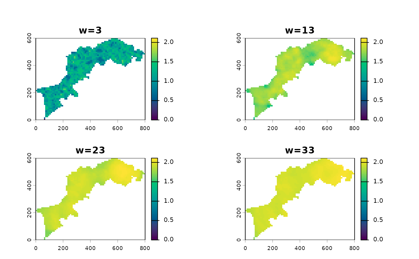p(l, global_range=FALSE) # each mono map has its scale

# change palette
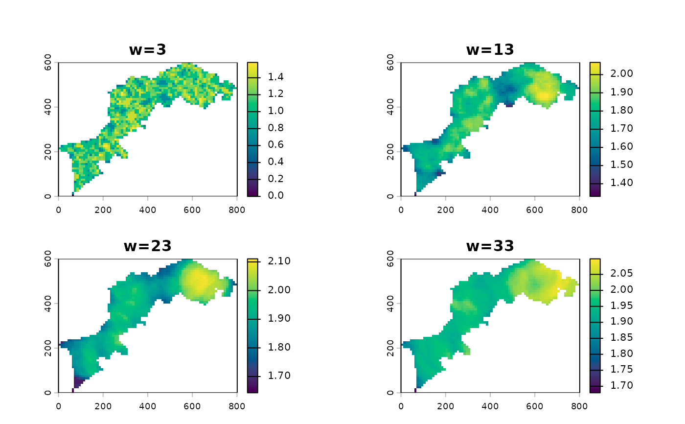
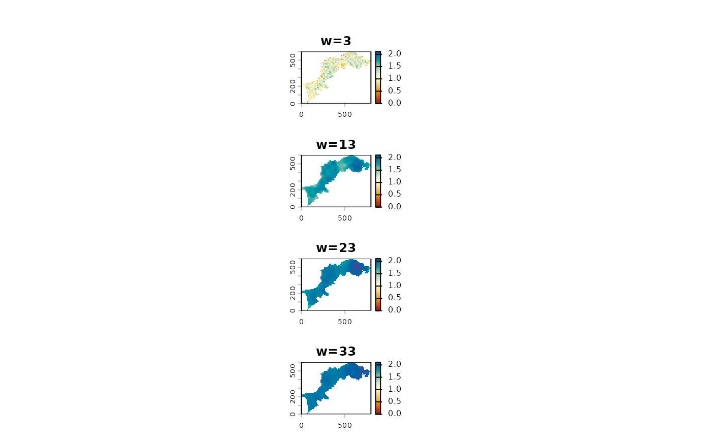
p(l, palette = "RdYlBu", ncol=1) # change the color palette for one of hcl.pals()


# manage title(s)
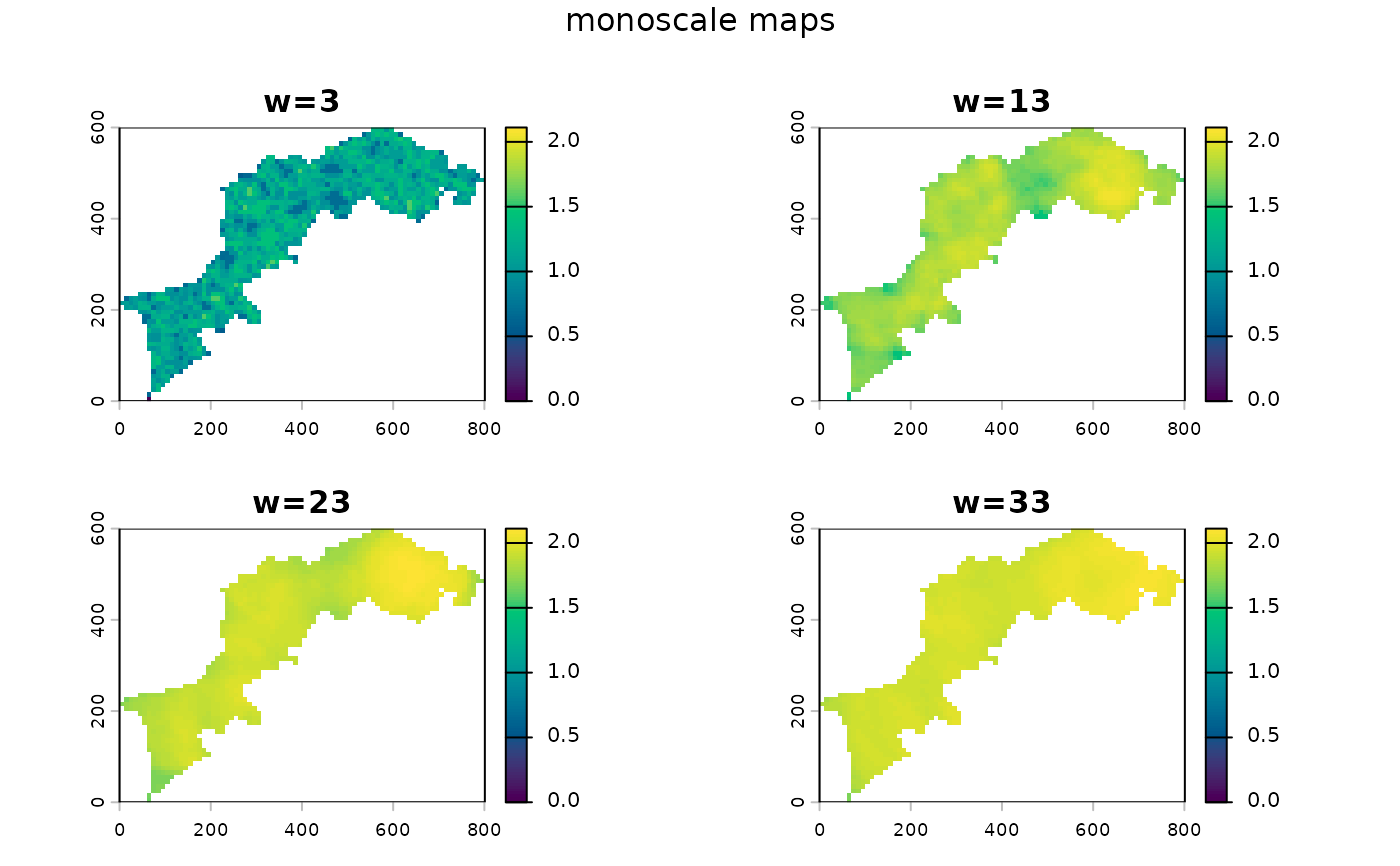
p(l, multi_title="monoscale maps")

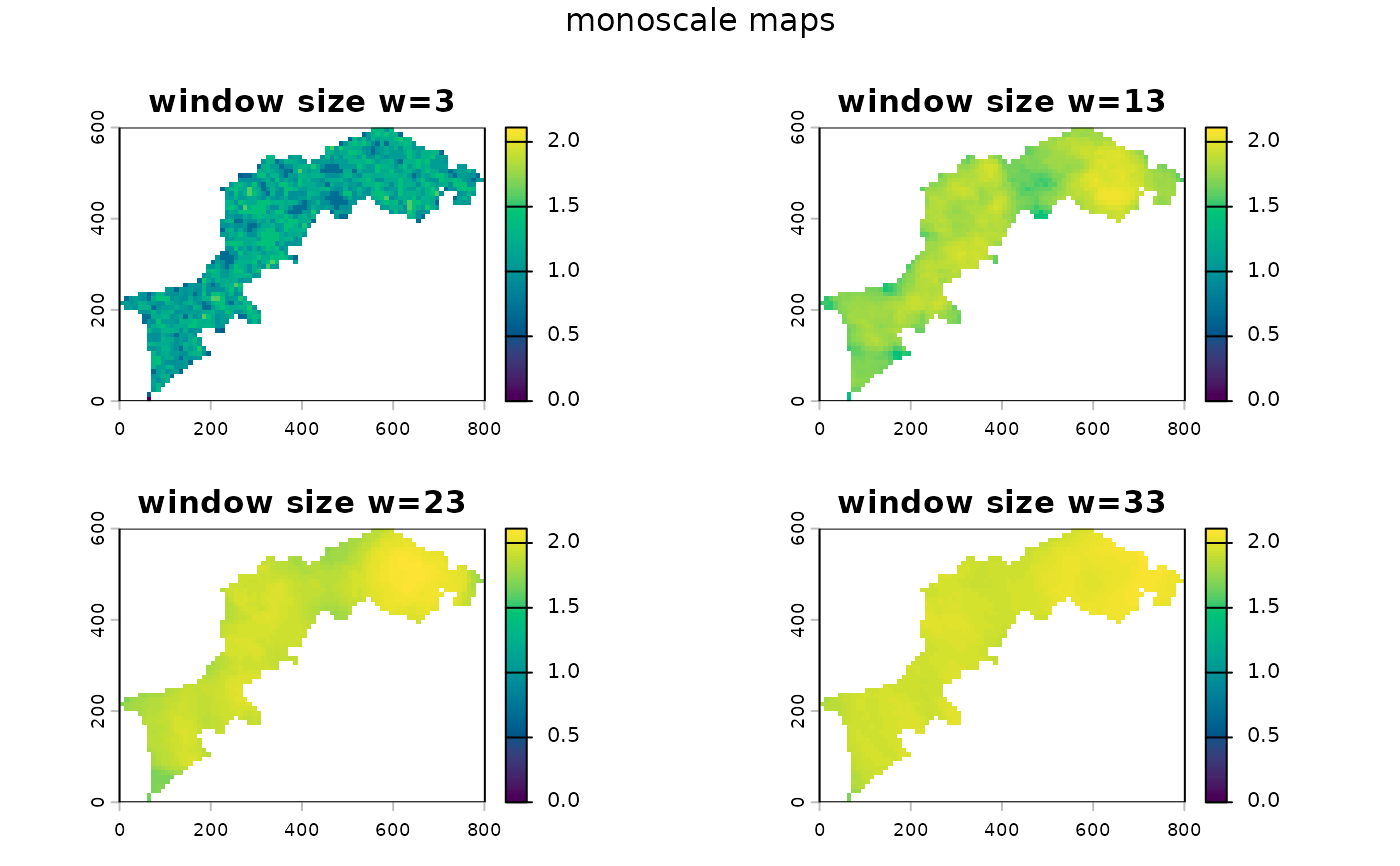
p(l, title=paste0("window size ", names(l)), multi_title="monoscale maps")


# change aspect
p(l, ncol=4)

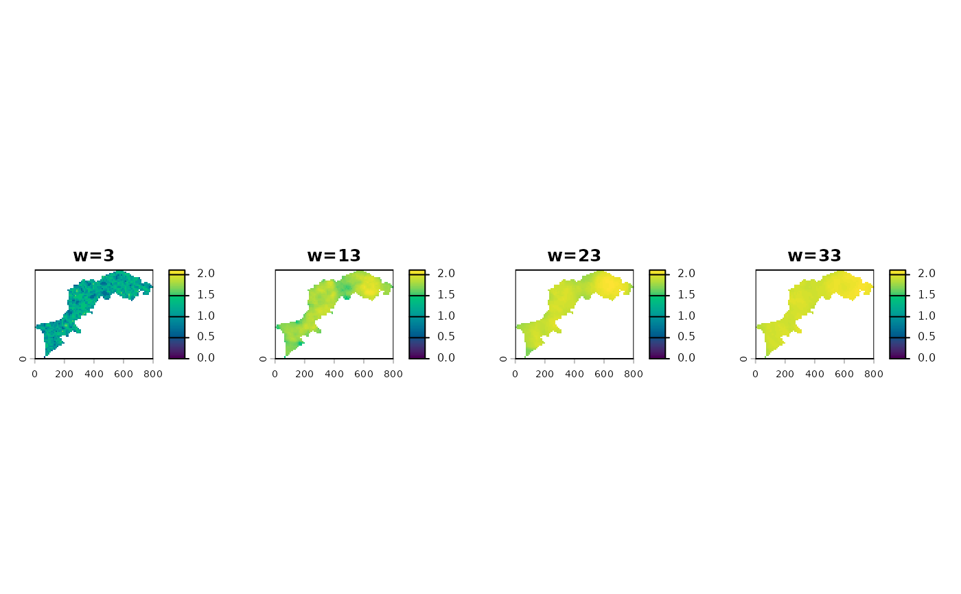p(l, ncol=1)