Description
Usage
CMP(
  x,
  y,
  window = window_quick(),
  kernel = kernel_circle,
  fun = mean,
  fillvalue = NA,
  ...
)
Arguments
- x, y
rasters as
terra::SpatRaster()- window
numeric sequence of window sizes (default to
c(3, 13, 23)via window_quick). Passed tokernelfunction- kernel
function among kernels (default to
kernel_circle)- fun
function that takes multiple numbers and return a single value such as
mean(default),median,min,max, terra::modal, richness, simpson, shannon, shannon_evenness or even custom functions (see vignette)- fillvalue
numeric. The value of the cells in the virtual rows and columns outside of the raster
- ...
additional parameters to pass to terra::focalPairs
References
Gaucherel, C., Alleaume, S. and Hély, C. (2008) The Comparison Map Profile method: a strategy for multiscale comparison of quantitative and qualitative images. IEEE Transactions on Geoscience and Remote Sensing 46 (9): 2708-2719 doi: 10.1109/TGRS.2008.919379
Examples
library(terra)
#> terra 1.8.86
# import the first example file
l1 <- import_example("l1.tif")
# and the second
l2 <- import_example("l2.tif")
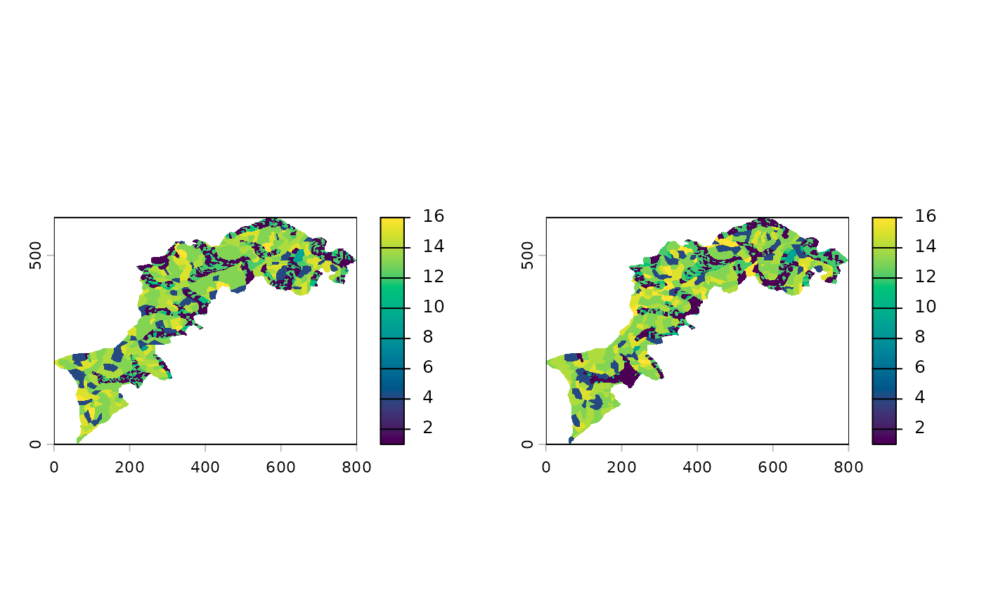
# we can plot them side by side
c(l1, l2) %>% p()
 # make them smaller by a factor 10 for example purpose
ls1 <- raster_resample(l1, 0.1)
ls2 <- raster_resample(l2, 0.1)
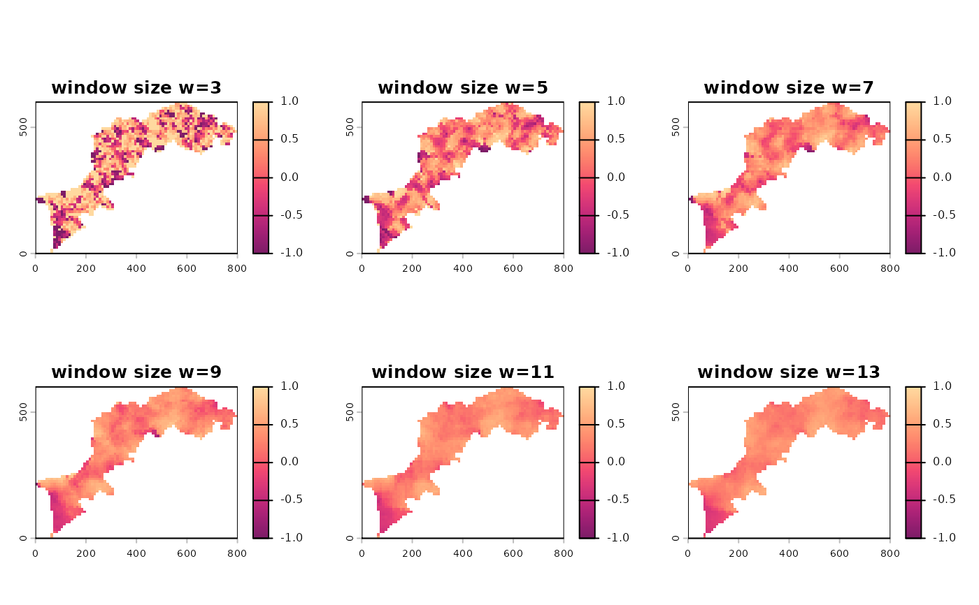
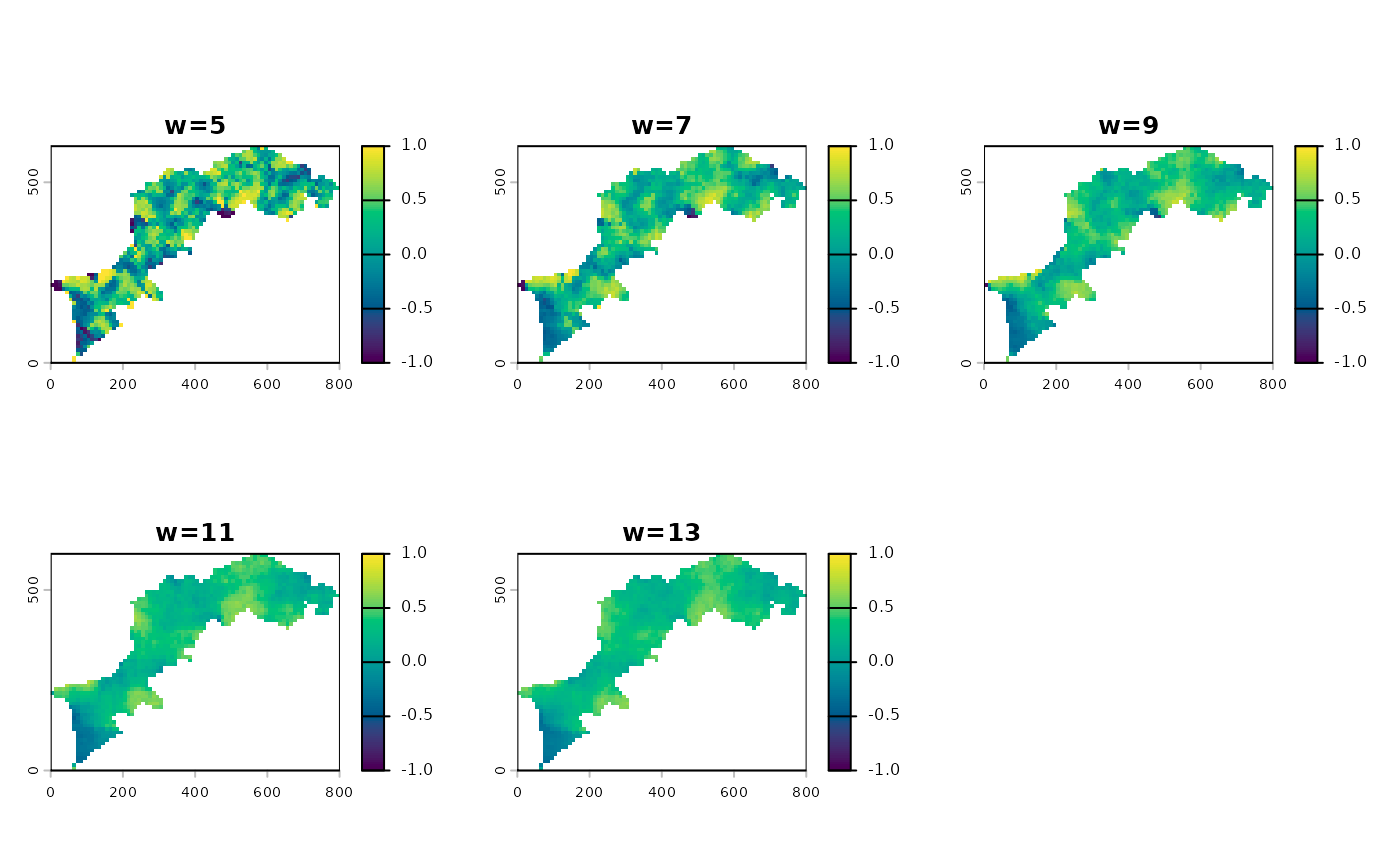
ls_cmp <- CMP(ls1, ls2,
window=seq(3, 13, by=2),
fun=cor_pearson)
# monoscale maps with customized title/palette
p(ls_cmp,
title=paste0("window size ", names(ls_cmp)),
palette="SunsetDark")
# make them smaller by a factor 10 for example purpose
ls1 <- raster_resample(l1, 0.1)
ls2 <- raster_resample(l2, 0.1)
ls_cmp <- CMP(ls1, ls2,
window=seq(3, 13, by=2),
fun=cor_pearson)
# monoscale maps with customized title/palette
p(ls_cmp,
title=paste0("window size ", names(ls_cmp)),
palette="SunsetDark")
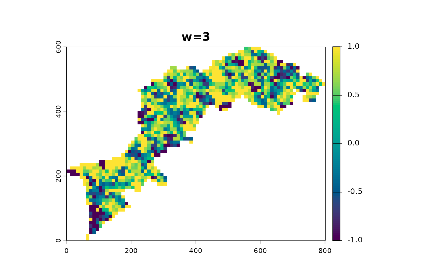
 # correlation is prone to NA when window is small enough
# to homogeneous focal values, ie with sd=0 and cor not defined.
# this gives us the opportunity to see how to select layers
p(ls_cmp[[1]])
# correlation is prone to NA when window is small enough
# to homogeneous focal values, ie with sd=0 and cor not defined.
# this gives us the opportunity to see how to select layers
p(ls_cmp[[1]])
 p(ls_cmp[[-1]])
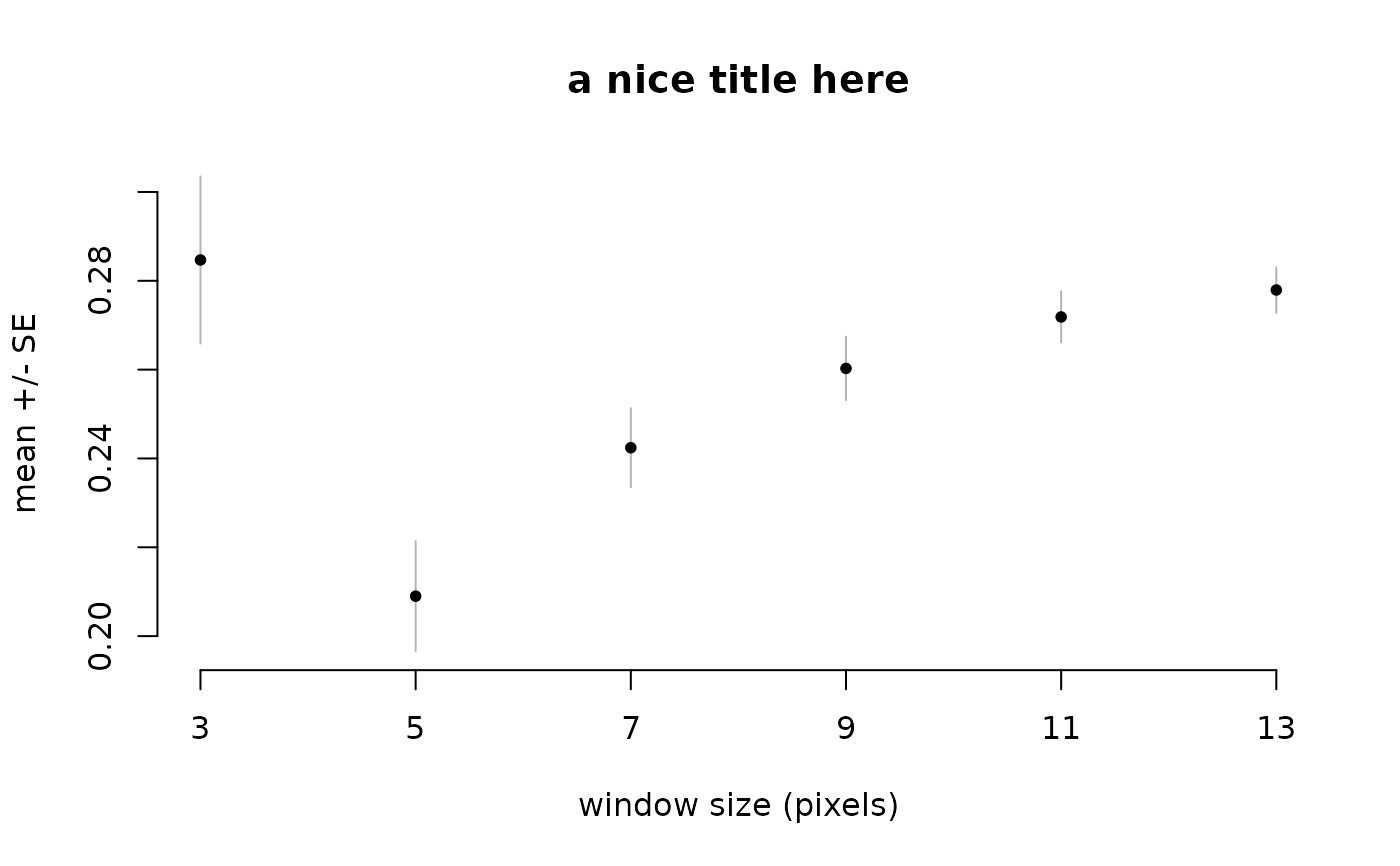
 # profile plot
ms_profile(ls_cmp, title="a nice title here")
# profile plot
ms_profile(ls_cmp, title="a nice title here")
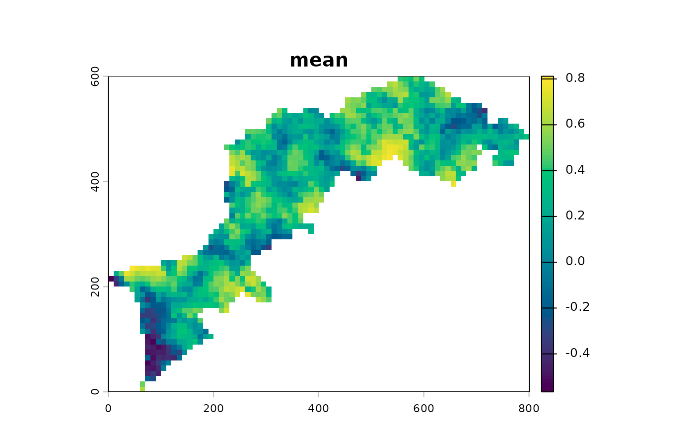
 app(ls_cmp, mean) %>% p()