3  Une introduction en 3 minutes

Le bloc de code ci-dessous combine tous les aspects que nous allons aborder dans ce document : utilisation de packages, du pipe %>%, préparation de données issues d’un tableau, production et customisation d’un graphe, création d’une fonction, calculs combinés sur listes de données, etc.

Comme pour tous les langages, naturels ou informatiques, vous parviendrez à déchiffrer avant d’écrire. D’autant que R est plus intransigeant qu’un autochtone en terre étrangère et ne laissera pas passer d’approximation.

Ceci étant, même si vous n’avez jamais vu de code R en action, ces commandes ainsi que les commentaires, précédés d’un # devraient être raisonnablement compréhensibles. Admirez la beauté du R “moderne”!

# dependencies
library(tidyverse)

# data tidying
# we will use the famous iris dataset
iris2 <- iris %>% 
  as_tibble() %>% 
  # only keep columns of interest
  select(pl=Petal.Length, pw=Petal.Width, sp=Species)
# let's print in on the console
iris2

# A tibble: 150 × 3
      pl    pw sp    
   <dbl> <dbl> <fct> 
 1   1.4   0.2 setosa
 2   1.4   0.2 setosa
 3   1.3   0.2 setosa
 4   1.5   0.2 setosa
 5   1.4   0.2 setosa
 6   1.7   0.4 setosa
 7   1.4   0.3 setosa
 8   1.5   0.2 setosa
 9   1.4   0.2 setosa
10   1.5   0.1 setosa
# ℹ 140 more rows

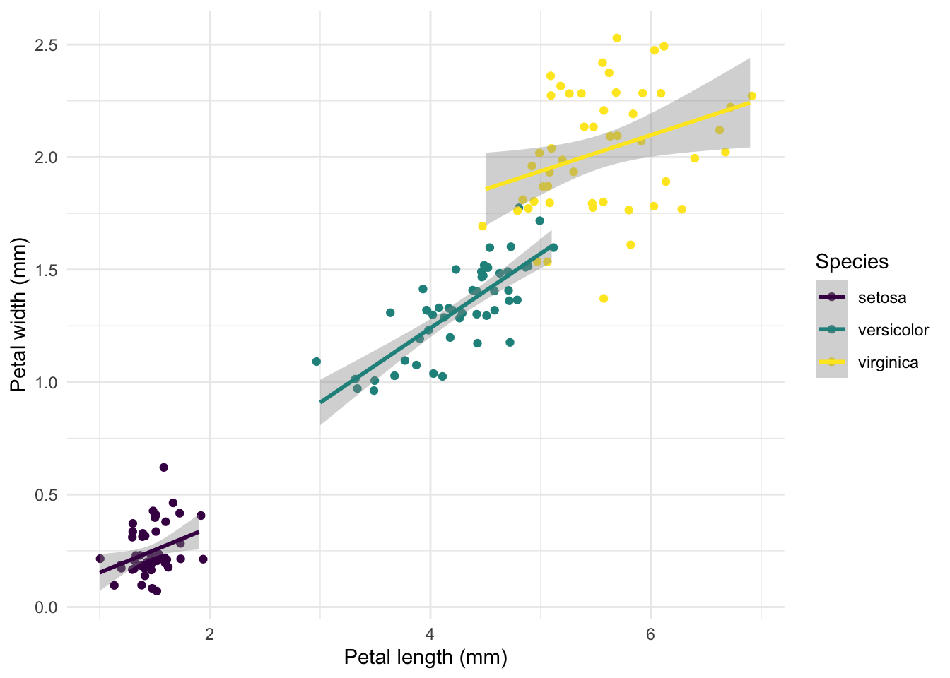
# a quick graph using ggplot2
# initialize using our dataset
ggplot(iris2) + 
  # define axes and columns to display
  aes(pl, pw, col=sp) + 
  # draw points, slightly jittered to show all 150 points
  geom_jitter() + 
  # let's add a linear model smooth
  geom_smooth(method="lm", formula="y~x") + 
  # here we tune colours
  scale_color_viridis_d() +
  # and add more cosmetics
  guides(colour=guide_legend("Species")) +
  xlab("Petal length (mm)") + ylab("Petal width (mm)") +
  # we love both cosmetics and minimal design
  theme_minimal()

# a little helper function to calculate a lm and extract the adjusted R2 from it
lm_adj_r2 <- function(x) summary(lm(pl~pw, data=x))$adj.r.squared
  
# let's adjust 3 linear models and extract adj R2
# group-wise statistics
iris2 %>%
  nest(data=c(pl, pw)) %>% 
  mutate(adj_r2=map_dbl(data, lm_adj_r2))

# A tibble: 3 × 3
  sp         data              adj_r2
  <fct>      <list>             <dbl>
1 setosa     <tibble [50 × 2]> 0.0914
2 versicolor <tibble [50 × 2]> 0.611 
3 virginica  <tibble [50 × 2]> 0.0851