Spaghetti plot after permutations

Display the result of permutations

Usage

spaghetti(df, x = x_pred, y = y_pred, by, size = 0.2, ...)

spaghetti0(
  df,
  x = x_new,
  y = y,
  by = NULL,
  method = NULL,
  formula = NULL,
  se = FALSE,
  size = 0.2,
  ...
)

Arguments

df

tibble() the result of a permutation function

x, y

colnames for x and y columns (x_new/y by default)

by

colnames for grouping column (optional, default to NULL)

size

passed to ggplot2::geom_line()/ggplot2::geom_smooth()

...

additional parameters to ggplot2::geom_line()/ggplot2::geom_smooth() (eg alpha) for spaghetti/spaghetti0, respectively

method, formula

passed ggplot2::geom_smooth(), and defaults to NULL so that we let ggplot2 pick default method when not specified

se

passed to ggplot2::geom_smooth(), default to FALSE to only draw lines

Details

This ggplot2 primer allows inspecting the effect of fitting functions (spaghetti) or raw data (spaghetti0).

Functions

• spaghetti: after quake and fit

• spaghetti0: straight after quake

Examples

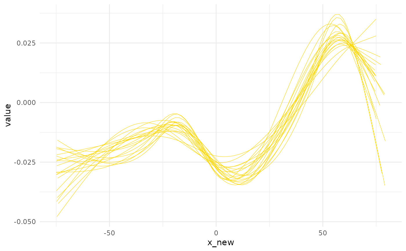
## spaghetti0 it the plotting function to use right after quake:

# general trend over permutations
spaghetti0(animals_q, x=x_new, y=value, col="gold")
#> `geom_smooth()` using method = 'gam' and formula 'y ~ s(x, bs = "cs")'


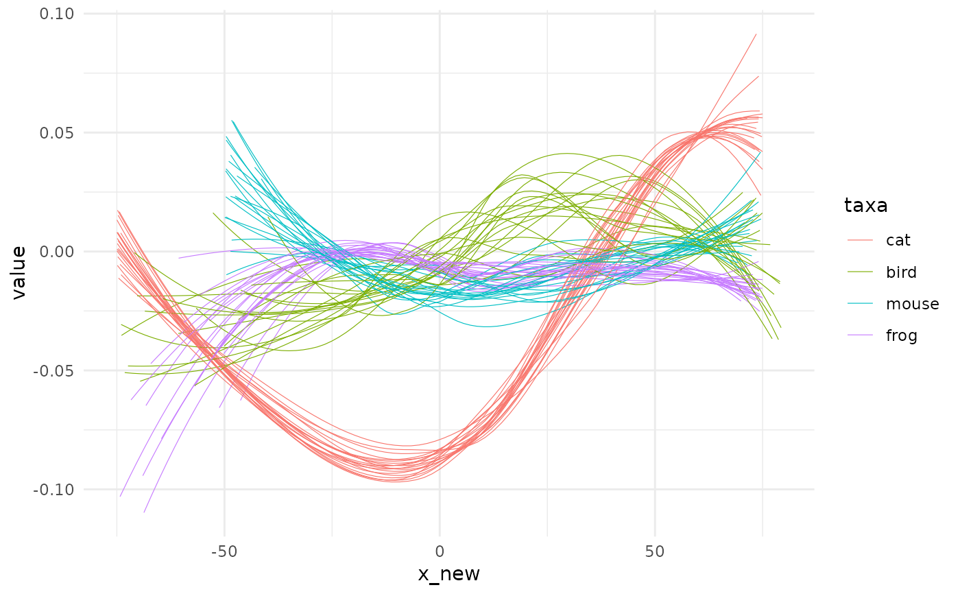
# per taxa now
spaghetti0(animals_q, x=x_new, y=value, by=taxa)
#> `geom_smooth()` using method = 'loess' and formula 'y ~ x'


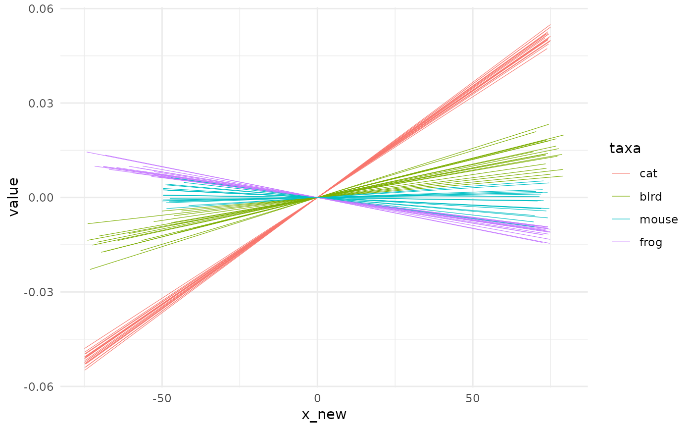
# you can choose other parameters for geom_smooth (if that makes sense)
# for instance, here lm with no intercept
spaghetti0(animals_q, x=x_new, y=value, by=taxa, method="lm", formula=y~x-1)


# you can also customise this using some ggplot2 spice
# note that if you library(ggplot2) you won't need all these ggplot2::
#' # color palette from https://www.colourlovers.com/palette/1473/Ocean_Five
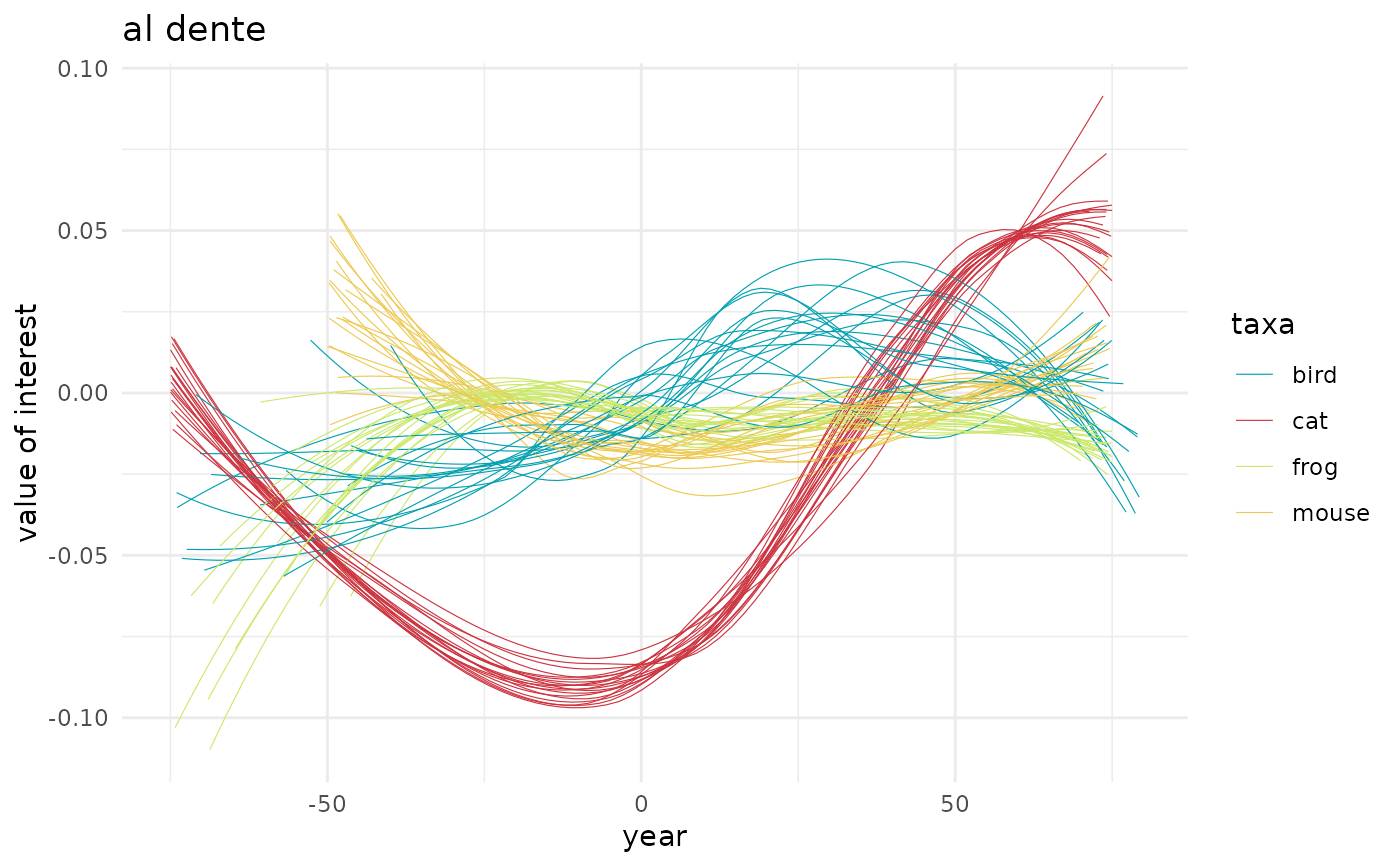
colors <- c("bird"="#00A0B0","cat"="#CC333F", "frog"="#CBE86B", "mouse"="#EDC951")
spaghetti0(animals_q, x=x_new, y=value, by=taxa) +
  ggplot2::scale_color_manual(values=colors) +
  ggplot2::labs(title="al dente", x="year", y="value of interest")
#> `geom_smooth()` using method = 'loess' and formula 'y ~ x'



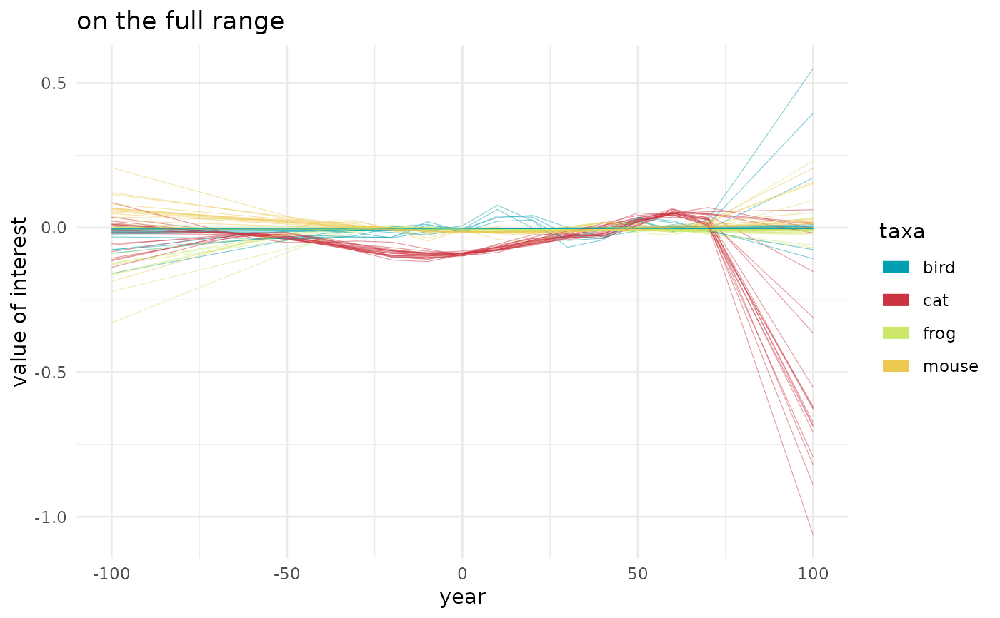
 ## spaghetti is intended for use _after_ fitting function
 ## it does not call geom_smooth but geom_line directly

 animals_f <- fit_gam(animals_q, y=value, by=taxa, x_pred=seq(-100, 100, 10))
#>  * fitting with gam(value ~ s(x_new, bs = "cs"))

 # and the general behaviour is the same as fo spaghetti0 eg:

 spaghetti(animals_f, by=taxa, alpha=0.5) +
  ggplot2::scale_color_manual(values=colors) +
  ggplot2::labs(title="on the full range", x="year", y="value of interest") +
  ggplot2::guides(colour=ggplot2::guide_legend(override.aes=list(size=3, alpha=1)))